
티스토리 뷰
Artificial Intelligence/Machine Learning
[ML] 다항회귀 (Polynomial regression)
inee0727 2022. 8. 19. 11:20다항 회귀 (Polynomial Regression)
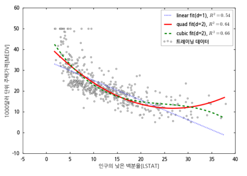
y=w0+w1x+w2x2+⋯+wdxd
- 독립변수의 차수를 높이는 형태
- 다차원의 회귀식인 다항 회귀 분석으로 단순 선형 모델의 한계를 어느정도 극복할 수 있음.
- 함수가 비선형, 데이터가 곡선 형태일 경우 예측에 유리
- 데이터에 각 특성의 제곱을 추가해주어서 특성이 추가된 비선형 데이터를 선형 회귀 모델로 훈련시키는 방법
- 보통 2차함수는 중간에 하강하므로 3차(cubic) 함수부터 아니면 단조증가하는 제곱근이나 로그 함수를 많이 쓴다.
- 다항 회귀도 결국 xd=Xd로 뒀을 때 다중 회귀식의 일종이라고 볼 수 있다.
%matplotlib inline
import numpy as np
import pandas as pd
import matplotlib
import matplotlib.pyplot as plt
from matplotlib import style
from sklearn.linear_model import LinearRegression
from sklearn.metrics import mean_squared_error
from sklearn.metrics import r2_score
from sklearn.preprocessing import PolynomialFeatures

style.use('seaborn-talk')
import matplotlib
import matplotlib.font_manager as fm
import os

# 한글 폰트 사용
def change_matplotlib_font(font_download_url):
    FONT_PATH = 'MY_FONT'

    font_download_cmd = f"wget {font_download_url} -O {FONT_PATH}.zip"
    unzip_cmd = f"unzip -o {FONT_PATH}.zip -d {FONT_PATH}"
    os.system(font_download_cmd)
    os.system(unzip_cmd)

    font_files = fm.findSystemFonts(fontpaths=FONT_PATH)
    for font_file in font_files:
        fm.fontManager.addfont(font_file)

    font_name = fm.FontProperties(fname=font_files[0]).get_name()
    matplotlib.rc('font', family=font_name)
    print("font family: ", plt.rcParams['font.family'])

font_download_url = "https://fonts.google.com/download?family=Noto%20Sans%20KR"
change_matplotlib_font(font_download_url)
# np.newaxis란 차원을 늘려줌 (10,)을 (10, 1)로
X = np.array([258, 270, 294, 320, 342,
368, 396, 446, 480, 586])[:, np.newaxis]
y = np.array([236.4, 234.4, 252.8, 298.6, 314.2,
342.2, 360.8, 368.0, 391.2, 390.8])
lr = LinearRegression()
pr = LinearRegression()
# 기본 다항식 형태 생성
# include_bias=True로 할 경우 0차항(1)도 함께 만든다. defualt값 True
quadratic = PolynomialFeatures(degree=2, include_bias=True)
# 정의된 numpy 배열은 행별로 각 데이터를 다항 형태로 변형해준다
# 1과 주어진 값과 주어진 값을 제곱한 항을 추가하여 반환
X_quad = quadratic.fit_transform(X)
display(X[0], X_quad[0]) # array([258]), array([1.0000e+00, 2.5800e+02, 6.6564e+04])
# 비교를 위해 단순 회귀 계산
lr.fit(X, y)
X_fit = np.arange(250, 600, 10)[:, np.newaxis]
y_lin_fit = lr.predict(X_fit)
# 다항 회귀를 위해 변형된 모델에 다중 회귀 모델 계산
pr.fit(X_quad, y)
y_quad_fit = pr.predict(quadratic.fit_transform(X_fit))
# 단순 회귀 및 다항 회귀 모델의 예측값 계산
y_lin_pred = lr.predict(X)
y_quad_pred = pr.predict(X_quad)
mse_lin = mean_squared_error(y, y_lin_pred)
mse_quad = mean_squared_error(y, y_quad_pred)
r2_lin = r2_score(y, y_lin_pred)
r2_quad = r2_score(y, y_quad_pred)
print(f'MSE\tLinear : {mse_lin:.2f},\tQuadratic: {mse_quad:.2f}')
print(f'R2\tLinear : {r2_lin:.2f},\tQuadratic: {r2_quad:.2f}')
plt.scatter(X, y, label='트레이닝 데이터')
plt.plot(X_fit, y_lin_fit, label='linear fit', linestyle='--')
plt.plot(X_fit, y_quad_fit, label='quadratic fit')
plt.legend(loc=2)
plt.show()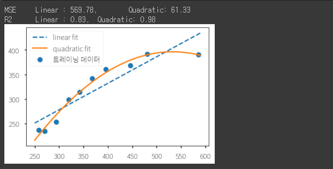
Pipeline 응용
위의 과정을 make_pipeline을 통해 PolynomialFeatures와 LinearRegression 과정이 한번에 통합된 모델을 생성
# 데이터 변환 과정과 머신러닝을 연결해주는 파이프라인
from sklearn.pipeline import make_pipeline

model_lr = make_pipeline(PolynomialFeatures(degree=2, include_bias=True),
						LinearRegression())
model_lr.fit(X, y)
print(model_lr.steps[1][1].coef_) # [ 0.00000000e+00  2.39893018e+00 -2.25020109e-03]
https://herjh0405.tistory.com/70
'Artificial Intelligence > Machine Learning' 카테고리의 다른 글
| [ML] 경사하강법(Gradient Descent) (1) | 2022.08.24 |
|---|---|
| [ML] ROC curve (0) | 2022.08.22 |
| [ML] XGBoost 개념 (0) | 2022.08.11 |
| [ML] 이상치(Outlier) 처리-(Tukey Outlier) (0) | 2022.08.10 |
| [ML] XGB plot_importance (0) | 2022.08.10 |